What Is Polynomial Regression In Machine Learning?
In a recent post i talked about linear regression with a practical python example. In this post we will analyze Polynomial regression and its use in data science as our next topic, because sometimes our data might not really be appropriate for a straight line. That’s where polynomial regression comes in.
In contrast with linear regression which follows the formula y = ax + b, polynomial regression follows the formula
y = anxn + an-1xn-1 + … + a1x + a0
The monomial anxn, an-1xn-1, …, a1x, a0 are called polynomial terms and the numbers an, an-1, …, a1, a0 are their coefficients. In particular, a0 is called fixed term of a polynomial.
So in other words, this type of regression is a form of linear regression in which the relationship between the independent variable x and dependent variable y is modeled as an nth degree polynomial.
For example, 2x3 – 5x2 + x – 2 is a 3rd degree polynomial, and -3x6 + 5x2 + 1 is a 6th degree polynomial.
Polynomial Regression Examples
It makes perfect sense that not always the relationship between our data points will be linear. Here are some quick examples.
- y = ax + b. This is a first degree polynomial, which is basically a linear one.
- y = ax2 + bx + c . This is a 2nd degree polynomial.
- y = ax3 + bx2 + cx + d. This is a 3rd degree polynomial.
- y = ax4 + bx3 + cx2 + dx + e. This is a 4rth degree polynomial.
Higher order produce more complex curves.
Things To Be Aware Of
- Don’t use more degrees than you actually need. Start from 2nd degree, and work your way up until you find the sweet spot that can predict future values.
- Visualize your data first to see how complex a curve might really be.
- Visualize the fit. Is your curve going out of its way to accommodate outliers?
- A high r-squared simply means your curve fits your training data well, but might not be a good predictor.
Usually there’s some natural relationship in our data that isn’t really all that complicated, and if we find ourselves throwing very large degrees at fitting our data, could made our model overfitting.
Practical Python Example
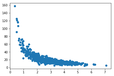
Let’s now take a look at some more real world data. For example page speed / purchase data:
%matplotlib inline
from pylab import *
import numpy as np

np.random.seed(2)
pageSpeed = np.random.normal(3.0, 1.0, 1000)
amountPurchased = np.random.normal(50.0, 10.0, 1000) / pageSpeed

scatter(pageSpeed, amountPurchased)
Output:
Fortunately for us, python module numpy has a handy polyfit function that we can take advantage of. It allows us generate a nth-degree polynomial model of our data set that minimizes squared errors. Let’s try it with a 5th degree polynomial and see what happens:
x = np.array(pageSpeed)
y = np.array(amountPurchased)

p4 = np.poly1d(np.polyfit(x, y, 5))
Now, we will visualize our original scatter plot, together with a plot of our predicted values using the polynomial for page speed times ranging from 0-7 seconds:
import matplotlib.pyplot as plt

xp = np.linspace(0, 7, 200)
plt.scatter(x, y)
plt.plot(xp, p4(xp), c='r')
plt.show()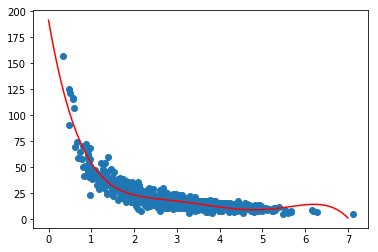
Looks pretty good! But let’s calculate the r-squared error our model has:
from sklearn.metrics import r2_score

r2 = r2_score(y, p4(x))
print(r2)
0.8553884386186101
85,54% accuracy, which is great, but not perfect!
Click to download the Jupyter notebook polynomial regression source code.
Alternately, you can view the contents on the current notebook online.