Multiple Regression Analysis In Machine Learning

Multiple Regression Analysis In Data Science

Let’s dive into multiple regression.

Multiple Regression That’s just a regression that takes more than one variable into account. More than one feature in our data set.

The concept is actually very simple. It’s just answering the question:

What if we have more than one variable, influencing the variable that we are trying to predict?

So basically we are doing a regression, that has more than one features, while we are attempting to calculate an other value.

There are many features that might come together. For an example that might be predicting the price of a car based on its many attributes. The car has a lot of different things you can measure that might influence its price such as its mileage, and its age, number of cylinders, and doors. We can then take all those into account, and roll that, into one big model that has many variables as part of it.

Often in Data Science, there is a confusing terminology.

In addition, we also have the concept of multivariate regression. Some people might think that is the same thing, but is not!

What Is The Difference Between Multiple And Multivariate Regression

A typical example, would be trying to predict not only the price of a car based on its mileage, age, and number of doors, but also trying to predict how much time it will take to sell it. So you can see that we have multiple variables that we are trying to predict in addition to multiple features being used to make those predictions.

Instead of having a single coefficient attached to a single feature variable, we have multiple terms, with multiple variables. So we can predict the price  variable, based on some constant value α, times some coefficient called β₁ first feature which say could be mileage, plus some coefficient β₂ which might be multiplying with some other feature like the age of the car, plus β₃ x number of doors. Those coefficients are just measuring how important each factor is, to the actual end result.

price = α + β₁ milage+ β₂ age + β₃ doors

This assumes that all of your features are normalized so you can actually compare those coefficients together fairly. If they’re not normalized, that coefficient will also be working to scale that feature, into the final result. And this could also be informative. If you actually discover the values of β₁, β₂, β₃, that can also tell you a little bit about what features are actually important for your model.

So if we end up with a very low coefficient for a given feature after everything are normalized, that might be a mathematical way of our model telling us that the given feature isn’t actually very important for predicting the value that we are trying to predict. And that can help us to simplify our model by eliminating feature data that we don’t really need. This is called “Feature Selection“, and is important for building a good machine learning model.

Practical Jupyter Notebook Example

This method still uses least squares. So in our notebook we’re going to use something called Ordinary Least Squares, and it can handle multiple features. So we can still measure overall the fit of the model using R-Squared. And another thing that we need to point out is that this whole thing assumes that there’s no dependency between these different features.

Notice that we treating all these features independently with their own coefficients. So if there is in fact a relationship between these features this model will not capture that. For example the mileage on a car would probably be highly correlated to the age of the car. And this model will not capture that relationship. Practically we will be just fine just using mileage or age independent of each other. But this could at least tell you which one of those is more important to keep.

Installing Necessary Python Packages

Before we begin, lets install some python packages needed for this example. These packages are pandas, statsmodels, and xlrd.

pip install pandas statsmodels xlrd

So lets create a practical example using Python, grabbing a data set of car values:

import pandas as pd

df = pd.read_excel('https://admintuts.net/wp-content/downloads/xls/cars.xls')
df.head()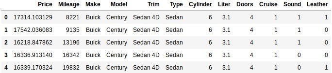

Out:

We’re gonna use Mapplotlib to visualize a graphical representation of our values. So we are gonna take all the values from mileage and price existing in this spreadsheet, and group these together into cars ranging from 0 – 50000 miles, with 10000 mile increments.

%matplotlib inline
import numpy as np

df1 = df[['Mileage','Price']]
bins =  np.arange(0,50000,10000)
groups = df1.groupby(pd.cut(df1['Mileage'],bins)).mean()

print(groups.head())
groups['Price'].plot.line()

Out:

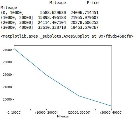
As you can see from the plot, its clear that as the mileage increases, the sale price decreases. Which makes perfect sense.

Now we will use pandas to split up this matrix into the feature vectors we care about, and the value we attempting to predict. Note that we are avoiding the make and model. Regressions don’t work well with ordinal values, unless you can convert them into some numerical order that makes sense to you.

Let’s scale our feature data into the same range, so we can easily compare the coefficients we will discover.

import statsmodels.api as sm
from sklearn.preprocessing import StandardScaler
scale = StandardScaler()

X = df[['Mileage', 'Cylinder', 'Doors']]
y = df['Price']

X[['Mileage', 'Cylinder', 'Doors']] = scale.fit_transform(X[['Mileage', 'Cylinder', 'Doors']].values())
print (X)
est = sm.OLS(y, X).fit()
est.summary()

Out:

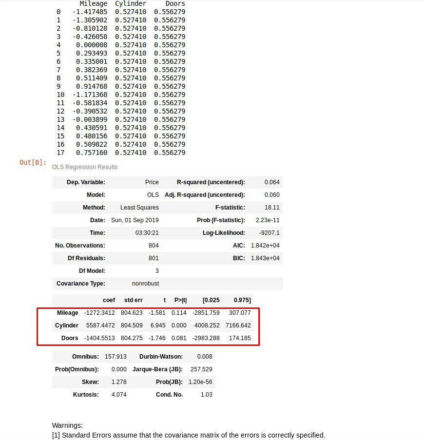
I highlighted the results that we are interested about because they they are rather interesting. It seems like the beta value that’s multiplied with the normalized mileage data, will contribute negative 1272 thousand to the final price.  The number of cylinders is positive 5587, and the number of doors is negative 1404.

y.groupby(df.Doors).mean()

Final Car Price Prediction Formula

scaled = scale.transform([[20000, 8, 4]])
predicted = est.predict(scaled[0])
print("Car predicted price is: ", *predicted, sep = "$")

Car predicted price is: $10198.259916713705